A Complete Tutorial on Tree Based Modeling from Scratch (in R & Python) from analytics vidya

Introduction

Tree based learning algorithms are considered to be one of the best and mostly used supervised learning methods. Tree based methods empower predictive models with high accuracy, stability and ease of interpretation. Unlike linear models, they map non-linear relationships quite well. They are adaptable at solving any kind of problem at hand (classification or regression).

Methods like decision trees, random forest, gradient boosting are being popularly used in all kinds of data science problems. Hence, for every analyst (fresher also), it’s important to learn these algorithms and use them for modeling.

This tutorial is meant to help beginners learn tree based modeling from scratch. After the successful completion of this tutorial, one is expected to become proficient at using tree based algorithms and build predictive models.

Note: This tutorial requires no prior knowledge of machine learning. However, elementary knowledge of R or Python will be helpful. To get started you can follow full tutorial in R and full tutorial in Python.

Table of Contents

1. What is a Decision Tree? How does it work?
2. Regression Trees vs Classification Trees
3. How does a tree decide where to split?
4. What are the key parameters of model building and how can we avoid over-fitting in decision trees?
5. Are tree based models better than linear models?
6. Working with Decision Trees in R and Python
7. What are the ensemble methods of trees based model?
8. What is Bagging? How does it work?
9. What is Random Forest ? How does it work?
10. What is Boosting ? How does it work?
11. Which is more powerful: GBM or Xgboost?
12. Working with GBM in R and Python
13. Working with Xgboost in R and Python
14. Where to Practice ?

1. What is a Decision Tree ? How does it work ?

Decision tree is a type of supervised learning algorithm (having a pre-defined target variable) that is mostly used in classification problems. It works for both categorical and continuous input and output variables. In this technique, we split the population or sample into two or more homogeneous sets (or sub-populations) based on most significant splitter / differentiator in input variables.

Example:-

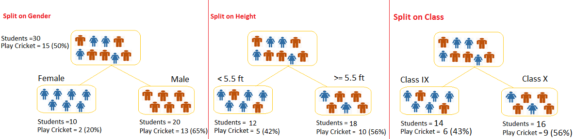
Let’s say we have a sample of 30 students with three variables Gender (Boy/ Girl), Class( IX/ X) and Height (5 to 6 ft). 15 out of these 30 play cricket in leisure time. Now, I want to create a model to predict who will play cricket during leisure period? In this problem, we need to segregate students who play cricket in their leisure time based on highly significant input variable among all three.

This is where decision tree helps, it will segregate the students based on all values of three variable and identify the variable, which creates the best homogeneous sets of students (which are heterogeneous to each other). In the snapshot below, you can see that variable Gender is able to identify best homogeneous sets compared to the other two variables.

As mentioned above, decision tree identifies the most significant variable and it’s value that gives best homogeneous sets of population. Now the question which arises is, how does it identify the variable and the split? To do this, decision tree uses various algorithms, which we will shall discuss in the following section.

Types of Decision Trees

Types of decision tree is based on the type of target variable we have. It can be of two types:

1. Categorical Variable Decision Tree: Decision Tree which has categorical target variable then it called as categorical variable decision tree. Example:- In above scenario of student problem, where the target variable was “Student will play cricket or not” i.e. YES or NO.
2. Continuous Variable Decision Tree: Decision Tree has continuous target variable then it is called as Continuous Variable Decision Tree.

Example:- Let’s say we have a problem to predict whether a customer will pay his renewal premium with an insurance company (yes/ no). Here we know that income of customer is a significant variable but insurance company does not have income details for all customers. Now, as we know this is an important variable, then we can build a decision tree to predict customer income based on occupation, product and various other variables. In this case, we are predicting values for continuous variable.

Important Terminology related to Decision Trees

Let’s look at the basic terminology used with Decision trees:

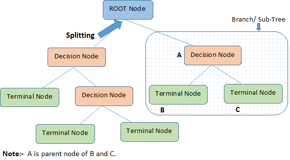
1. Root Node: It represents entire population or sample and this further gets divided into two or more homogeneous sets.
2. Splitting: It is a process of dividing a node into two or more sub-nodes.
3. Decision Node: When a sub-node splits into further sub-nodes, then it is called decision node.
4. Leaf/ Terminal Node: Nodes do not split is called Leaf or Terminal node.
5. Pruning: When we remove sub-nodes of a decision node, this process is called pruning. You can say opposite process of splitting.
6. Branch / Sub-Tree: A sub section of entire tree is called branch or sub-tree.
7. Parent and Child Node: A node, which is divided into sub-nodes is called parent node of sub-nodes where as sub-nodes are the child of parent node.

These are the terms commonly used for decision trees. As we know that every algorithm has advantages and disadvantages, below are the important factors which one should know.

Advantages

1. Easy to Understand: Decision tree output is very easy to understand even for people from non-analytical background. It does not require any statistical knowledge to read and interpret them. Its graphical representation is very intuitive and users can easily relate their hypothesis.
2. Useful in Data exploration: Decision tree is one of the fastest way to identify most significant variables and relation between two or more variables. With the help of decision trees, we can create new variables / features that has better power to predict target variable. You can refer article (Trick to enhance power of regression model) for one such trick.  It can also be used in data exploration stage. For example, we are working on a problem where we have information available in hundreds of variables, there decision tree will help to identify most significant variable.
3. Less data cleaning required: It requires less data cleaning compared to some other modeling techniques. It is not influenced by outliers and missing values to a fair degree.
4. Data type is not a constraint: It can handle both numerical and categorical variables.
5. Non Parametric Method: Decision tree is considered to be a non-parametric method. This means that decision trees have no assumptions about the space distribution and the classifier structure.

Disadvantages

1. Over fitting: Over fitting is one of the most practical difficulty for decision tree models. This problem gets solved by setting constraints on model parameters and pruning (discussed in detailed below).
2. Not fit for continuous variables: While working with continuous numerical variables, decision tree looses information when it categorizes variables in different categories.

2. Regression Trees vs Classification Trees

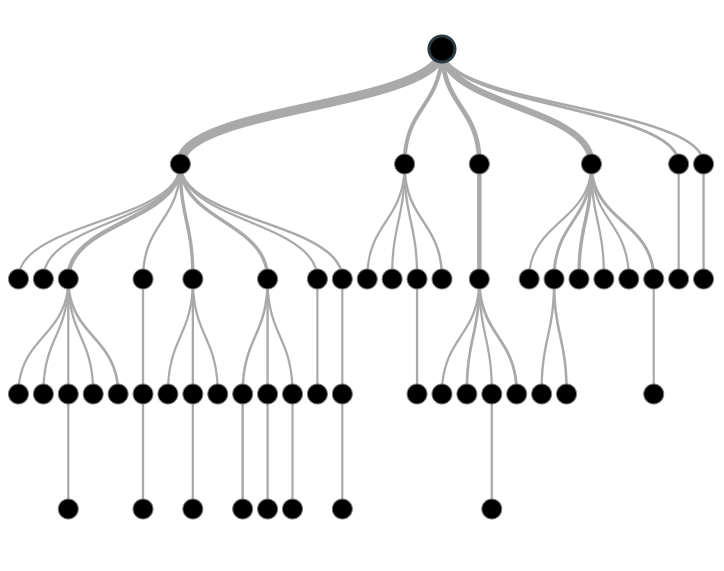
We all know that the terminal nodes (or leaves) lies at the bottom of the decision tree. This means that decision trees are typically drawn upside down such that leaves are the the bottom & roots are the tops (shown below).

Both the trees work almost similar to each other, let’s look at the primary differences & similarity between classification and regression trees:

1. Regression trees are used when dependent variable is continuous. Classification trees are used when dependent variable is categorical.
2. In case of regression tree, the value obtained by terminal nodes in the training data is the mean response of observation falling in that region. Thus, if an unseen data observation falls in that region, we’ll make its prediction with mean value.
3. In case of classification tree, the value (class) obtained by terminal node in the training data is the mode of observations falling in that region. Thus, if an unseen data observation falls in that region, we’ll make its prediction with mode value.
4. Both the trees divide the predictor space (independent variables) into distinct and non-overlapping regions. For the sake of simplicity, you can think of these regions as high dimensional boxes or boxes.
5. Both the trees follow a top-down greedy approach known as recursive binary splitting. We call it as ‘top-down’ because it begins from the top of tree when all the observations are available in a single region and successively splits the predictor space into two new branches down the tree. It is known as ‘greedy’ because, the algorithm cares (looks for best variable available) about only the current split, and not about future splits which will lead to a better tree.
6. This splitting process is continued until a user defined stopping criteria is reached. For example: we can tell the the algorithm to stop once the number of observations per node becomes less than 50.
7. In both the cases, the splitting process results in fully grown trees until the stopping criteria is reached. But, the fully grown tree is likely to overfit data, leading to poor accuracy on unseen data. This bring ‘pruning’. Pruning is one of the technique used tackle overfitting. We’ll learn more about it in following section.

3. How does a tree decide where to split?

The decision of making strategic splits heavily affects a tree’s accuracy. The decision criteria is different for classification and regression trees.

Decision trees use multiple algorithms to decide to split a node in two or more sub-nodes. The creation of sub-nodes increases the homogeneity of resultant sub-nodes. In other words, we can say that purity of the node increases with respect to the target variable. Decision tree splits the nodes on all available variables and then selects the split which results in most homogeneous sub-nodes.

The algorithm selection is also based on type of target variables. Let’s look at the four most commonly used algorithms in decision tree:

Gini Index

Gini index says, if we select two items from a population at random then they must be of same class and probability for this is 1 if population is pure.

1. It works with categorical target variable “Success” or “Failure”.
2. It performs only Binary splits
3. Higher the value of Gini higher the homogeneity.
4. CART (Classification and Regression Tree) uses Gini method to create binary splits.

Steps to Calculate Gini for a split

1. Calculate Gini for sub-nodes, using formula sum of square of probability for success and failure (p^2+q^2).
2. Calculate Gini for split using weighted Gini score of each node of that split

Example: – Referring to example used above, where we want to segregate the students based on target variable ( playing cricket or not ). In the snapshot below, we split the population using two input variables Gender and Class. Now, I want to identify which split is producing more homogeneous sub-nodes using Gini index.

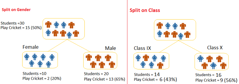Split on Gender:

1. Calculate, Gini for sub-node Female = (0.2)*(0.2)+(0.8)*(0.8)=0.68
2. Gini for sub-node Male = (0.65)*(0.65)+(0.35)*(0.35)=0.55
3. Calculate weighted Gini for Split Gender = (10/30)*0.68+(20/30)*0.55 = 0.59

Similar for Split on Class:

1. Gini for sub-node Class IX = (0.43)*(0.43)+(0.57)*(0.57)=0.51
2. Gini for sub-node Class X = (0.56)*(0.56)+(0.44)*(0.44)=0.51
3. Calculate weighted Gini for Split Class = (14/30)*0.51+(16/30)*0.51 = 0.51

Above, you can see that Gini score for Split on Gender is higher than Split on Class, hence, the node split will take place on Gender.

Chi-Square

It is an algorithm to find out the statistical significance between the differences between sub-nodes and parent node. We measure it by sum of squares of standardized differences between observed and expected frequencies of target variable.

1. It works with categorical target variable “Success” or “Failure”.
2. It can perform two or more splits.
3. Higher the value of Chi-Square higher the statistical significance of differences between sub-node and Parent node.
4. Chi-Square of each node is calculated using formula,
5. Chi-square = ((Actual – Expected)^2 / Expected)^1/2
6. It generates tree called CHAID (Chi-square Automatic Interaction Detector)

Steps to Calculate Chi-square for a split:

1. Calculate Chi-square for individual node by calculating the deviation for Success and Failure both
2. Calculated Chi-square of Split using Sum of all Chi-square of success and Failure of each node of the split

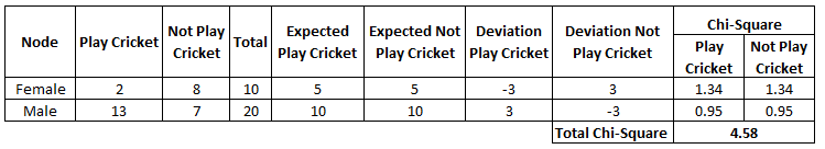
Example: Let’s work with above example that we have used to calculate Gini.

Split on Gender:

1. First we are populating for node Female, Populate the actual value for “Play Cricket” and “Not Play Cricket”, here these are 2 and 8 respectively.
2. Calculate expected value for “Play Cricket” and “Not Play Cricket”, here it would be 5 for both because parent node has probability of 50% and we have applied same probability on Female count(10).
3. Calculate deviations by using formula, Actual – Expected. It is for “Play Cricket” (2 – 5 = -3) and for “Not play cricket” ( 8 – 5 = 3).
4. Calculate Chi-square of node for “Play Cricket” and “Not Play Cricket” using formula with formula, = ((Actual – Expected)^2 / Expected)^1/2. You can refer below table for calculation.
5. Follow similar steps for calculating Chi-square value for Male node.
6. Now add all Chi-square values to calculate Chi-square for split Gender.

Split on Class:

Perform similar steps of calculation for split on Class and you will come up with below table.

Above, you can see that Chi-square also identify the Gender split is more significant compare to Class.

Information Gain:

Look at the image below and think which node can be described easily. I am sure, your answer is C because it requires less information as all values are similar. On the other hand, B requires more information to describe it and A requires the maximum information. In other words, we can say that C is a Pure node, B is less Impure and A is more impure.

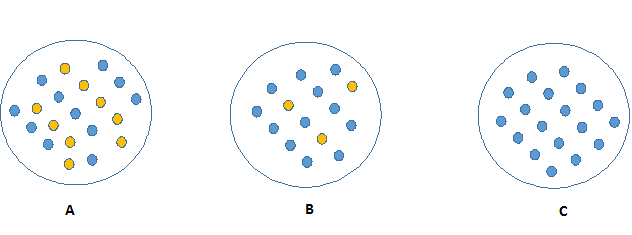
Now, we can build a conclusion that less impure node requires less information to describe it. And, more impure node requires more information. Information theory is a measure to define this degree of disorganization in a system known as Entropy. If the sample is completely homogeneous, then the entropy is zero and if the sample is an equally divided (50% – 50%), it has entropy of one.

Entropy can be calculated using formula:-

Here p and q is probability of success and failure respectively in that node. Entropy is also used with categorical target variable. It chooses the split which has lowest entropy compared to parent node and other splits. The lesser the entropy, the better it is.

Steps to calculate entropy for a split:

1. Calculate entropy of parent node
2. Calculate entropy of each individual node of split and calculate weighted average of all sub-nodes available in split.

Example: Let’s use this method to identify best split for student example.

1. Entropy for parent node = -(15/30) log2 (15/30) – (15/30) log2 (15/30) = 1. Here 1 shows that it is a impure node.
2. Entropy for Female node = -(2/10) log2 (2/10) – (8/10) log2 (8/10) = 0.72 and for male node,  -(13/20) log2 (13/20) – (7/20) log2 (7/20) = 0.93
3. Entropy for split Gender = Weighted entropy of sub-nodes = (10/30)*0.72 + (20/30)*0.93 = 0.86
4. Entropy for Class IX node, -(6/14) log2 (6/14) – (8/14) log2 (8/14) = 0.99 and for Class X node,  -(9/16) log2 (9/16) – (7/16) log2 (7/16) = 0.99.
5. Entropy for split Class =  (14/30)*0.99 + (16/30)*0.99 = 0.99

Above, you can see that entropy for Split on Gender is the lowest among all, so the tree will split on Gender. We can derive information gain from entropy as 1- Entropy.

Reduction in Variance

Till now, we have discussed the algorithms for categorical target variable. Reduction in variance is an algorithm used for continuous target variables (regression problems). This algorithm uses the standard formula of variance to choose the best split. The split with lower variance is selected as the criteria to split the population:

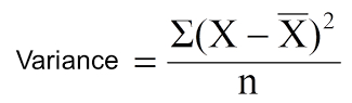
Above X-bar is mean of the values, X is actual and n is number of values.

Steps to calculate Variance:

1. Calculate variance for each node.
2. Calculate variance for each split as weighted average of each node variance.

Example:- Let’s assign numerical value 1 for play cricket and 0 for not playing cricket. Now follow the steps to identify the right split:

1. Variance for Root node, here mean value is (15*1 + 15*0)/30 = 0.5 and we have 15 one and 15 zero. Now variance would be ((1-0.5)^2+(1-0.5)^2+….15 times+(0-0.5)^2+(0-0.5)^2+…15 times) / 30, this can be written as (15*(1-0.5)^2+15*(0-0.5)^2) / 30 = 0.25
2. Mean of Female node =  (2*1+8*0)/10=0.2 and Variance = (2*(1-0.2)^2+8*(0-0.2)^2) / 10 = 0.16
3. Mean of Male Node = (13*1+7*0)/20=0.65 and Variance = (13*(1-0.65)^2+7*(0-0.65)^2) / 20 = 0.23
4. Variance for Split Gender = Weighted Variance of Sub-nodes = (10/30)*0.16 + (20/30) *0.23 = 0.21
5. Mean of Class IX node =  (6*1+8*0)/14=0.43 and Variance = (6*(1-0.43)^2+8*(0-0.43)^2) / 14= 0.24
6. Mean of Class X node =  (9*1+7*0)/16=0.56 and Variance = (9*(1-0.56)^2+7*(0-0.56)^2) / 16 = 0.25
7. Variance for Split Gender = (14/30)*0.24 + (16/30) *0.25 = 0.25

Above, you can see that Gender split has lower variance compare to parent node, so the split would take place on Gender variable.

Until here, we learnt about the basics of decision trees and the decision making process involved to choose the best splits in building a tree model. As I said, decision tree can be applied both on regression and classification problems. Let’s understand these aspects in detail.

4. What are the key parameters of tree modeling and how can we avoid over-fitting in decision trees?

Overfitting is one of the key challenges faced while modeling decision trees. If there is no limit set of a decision tree, it will give you 100% accuracy on training set because in the worse case it will end up making 1 leaf for each observation. Thus, preventing overfitting is pivotal while modeling a decision tree and it can be done in 2 ways:

1. Setting constraints on tree size
2. Tree pruning

Lets discuss both of these briefly.

Setting Constraints on Tree Size

This can be done by using various parameters which are used to define a tree. First, lets look at the general structure of a decision tree:

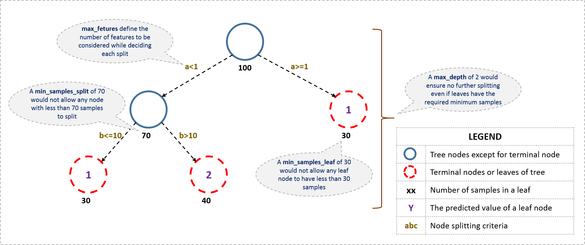
The parameters used for defining a tree are further explained below. The parameters described below are irrespective of tool. It is important to understand the role of parameters used in tree modeling. These parameters are available in R & Python.

1. Minimum samples for a node split
   • Defines the minimum number of samples (or observations) which are required in a node to be considered for splitting.
   • Used to control over-fitting. Higher values prevent a model from learning relations which might be highly specific to the particular sample selected for a tree.
   • Too high values can lead to under-fitting hence, it should be tuned using CV.
2. Minimum samples for a terminal node (leaf)
   • Defines the minimum samples (or observations) required in a terminal node or leaf.
   • Used to control over-fitting similar to min_samples_split.
   • Generally lower values should be chosen for imbalanced class problems because the regions in which the minority class will be in majority will be very small.
3. Maximum depth of tree (vertical depth)
   • The maximum depth of a tree.
   • Used to control over-fitting as higher depth will allow model to learn relations very specific to a particular sample.
   • Should be tuned using CV.
4. Maximum number of terminal nodes
   • The maximum number of terminal nodes or leaves in a tree.
   • Can be defined in place of max_depth. Since binary trees are created, a depth of ‘n’ would produce a maximum of 2^n leaves.
5. Maximum features to consider for split
   • The number of features to consider while searching for a best split. These will be randomly selected.
   • As a thumb-rule, square root of the total number of features works great but we should check upto 30-40% of the total number of features.
   • Higher values can lead to over-fitting but depends on case to case.

Tree Pruning

As discussed earlier, the technique of setting constraint is a greedy-approach. In other words, it will check for the best split instantaneously and move forward until one of the specified stopping condition is reached. Let’s consider the following case when you’re driving:

There are 2 lanes:

1. A lane with cars moving at 80km/h
2. A lane with trucks moving at 30km/h

At this instant, you are the yellow car and you have 2 choices:

1. Take a left and overtake the other 2 cars quickly
2. Keep moving in the present lane

Lets analyze these choice. In the former choice, you’ll immediately overtake the car ahead and reach behind the truck and start moving at 30 km/h, looking for an opportunity to move back right. All cars originally behind you move ahead in the meanwhile. This would be the optimum choice if your objective is to maximize the distance covered in next say 10 seconds. In the later choice, you sale through at same speed, cross trucks and then overtake maybe depending on situation ahead. Greedy you!

This is exactly the difference between normal decision tree & pruning. A decision tree with constraints won’t see the truck ahead and adopt a greedy approach by taking a left. On the other hand if we use pruning, we in effect look at a few steps ahead and make a choice.

So we know pruning is better. But how to implement it in decision tree? The idea is simple.

1. We first make the decision tree to a large depth.
2. Then we start at the bottom and start removing leaves which are giving us negative returns when compared from the top.
3. Suppose a split is giving us a gain of say -10 (loss of 10) and then the next split on that gives us a gain of 20. A simple decision tree will stop at step 1 but in pruning, we will see that the overall gain is +10 and keep both leaves.

Note that sklearn’s decision tree classifier does not currently support pruning. Advanced packages like xgboost have adopted tree pruning in their implementation. But the library rpart in R, provides a function to prune. Good for R users!

5. Are tree based models better than linear models?

“If I can use logistic regression for classification problems and linear regression for regression problems, why is there a need to use trees”? Many of us have this question. And, this is a valid one too.

Actually, you can use any algorithm. It is dependent on the type of problem you are solving. Let’s look at some key factors which will help you to decide which algorithm to use:

1. If the relationship between dependent & independent variable is well approximated by a linear model, linear regression will outperform tree based model.
2. If there is a high non-linearity & complex relationship between dependent & independent variables, a tree model will outperform a classical regression method.
3. If you need to build a model which is easy to explain to people, a decision tree model will always do better than a linear model. Decision tree models are even simpler to interpret than linear regression!

6. Working with Decision Trees in R and Python

For R users and Python users, decision tree is quite easy to implement. Let’s quickly look at the set of codes which can get you started with this algorithm. For ease of use, I’ve shared standard codes where you’ll need to replace your data set name and variables to get started.

For R users, there are multiple packages available to implement decision tree such as ctree, rpart, tree etc.

> library(rpart)
> x <- cbind="" class="c" span="" style="box-sizing: border-box;" x_train="" y_train=""># grow tree 
> fit <- rpart="" span="">y_train ~ ., data = x,method="class")
> summary(fit)
#Predict Output 
> predicted= predict(fit,x_test)

In the code above:

• y_train – represents dependent variable.
• x_train – represents independent variable
• x – represents training data.

For Python users, below is the code:

#Import Library
#Import other necessary libraries like pandas, numpy...
from sklearn import tree
#Assumed you have, X (predictor) and Y (target) for training data set and x_test(predictor) of test_dataset
# Create tree object 
model = tree.DecisionTreeClassifier(criterion='gini') # for classification, here you can change the algorithm as gini or entropy (information gain) by default it is gini  
# model = tree.DecisionTreeRegressor() for regression
# Train the model using the training sets and check score
model.fit(X, y)
model.score(X, y)
#Predict Output
predicted= model.predict(x_test)

7. What are ensemble methods in tree based modeling ?

The literary meaning of word ‘ensemble’ is group. Ensemble methods involve group of predictive models to achieve a better accuracy and model stability. Ensemble methods are known to impart supreme boost to tree based models.

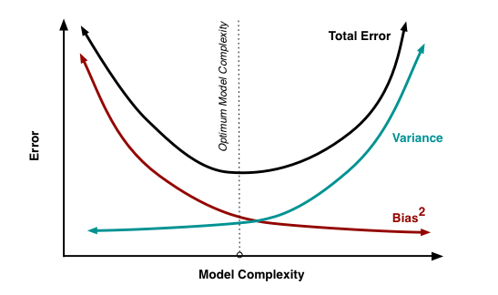
Like every other model, a tree based model also suffers from the plague of bias and variance. Bias means, ‘how much on an average are the predicted values different from the actual value.’ Variance means, ‘how different will the predictions of the model be at the same point if different samples are taken from the same population’.

You build a small tree and you will get a model with low variance and high bias. How do you manage to balance the trade off between bias and variance ?

Normally, as you increase the complexity of your model, you will see a reduction in prediction error due to lower bias in the model. As you continue to make your model more complex, you end up over-fitting your model and your model will start suffering from high variance.

A champion model should maintain a balance between these two types of errors. This is known as the trade-off management of bias-variance errors. Ensemble learning is one way to execute this trade off analysis.

Some of the commonly used ensemble methods include: Bagging, Boosting and Stacking. In this tutorial, we’ll focus on Bagging and Boosting in detail.

8. What is Bagging? How does it work?

Bagging is a technique used to reduce the variance of our predictions by combining the result of multiple classifiers modeled on different sub-samples of the same data set. The following figure will make it clearer:

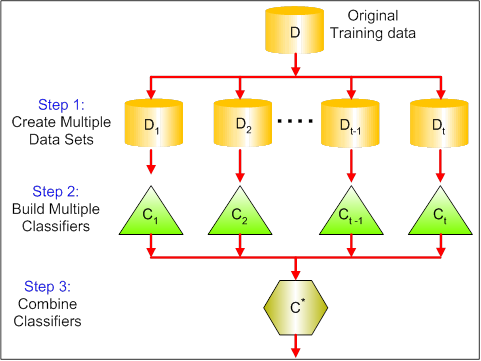
The steps followed in bagging are:

1. Create Multiple DataSets:
   • Sampling is done with replacement on the original data and new datasets are formed.
   • The new data sets can have a fraction of the columns as well as rows, which are generally hyper-parameters in a bagging model
   • Taking row and column fractions less than 1 helps in making robust models, less prone to overfitting
2. Build Multiple Classifiers:
   • Classifiers are built on each data set.
   • Generally the same classifier is modeled on each data set and predictions are made.
3. Combine Classifiers:
   • The predictions of all the classifiers are combined using a mean, median or mode value depending on the problem at hand.
   • The combined values are generally more robust than a single model.

Note that, here the number of models built is not a hyper-parameters. Higher number of models are always better or may give similar performance than lower numbers. It can be theoretically shown that the variance of the combined predictions are reduced to 1/n (n: number of classifiers) of the original variance, under some assumptions.

There are various implementations of bagging models. Random forest is one of them and we’ll discuss it next.

9. What is Random Forest ? How does it work?

Random Forest is considered to be a panacea of all data science problems. On a funny note, when you can’t think of any algorithm (irrespective of situation), use random forest!

Random Forest is a versatile machine learning method capable of performing both regression and classification tasks. It also undertakes dimensional reduction methods, treats missing values, outlier values and other essential steps of data exploration, and does a fairly good job. It is a type of ensemble learning method, where a group of weak models combine to form a powerful model.

How does it work?

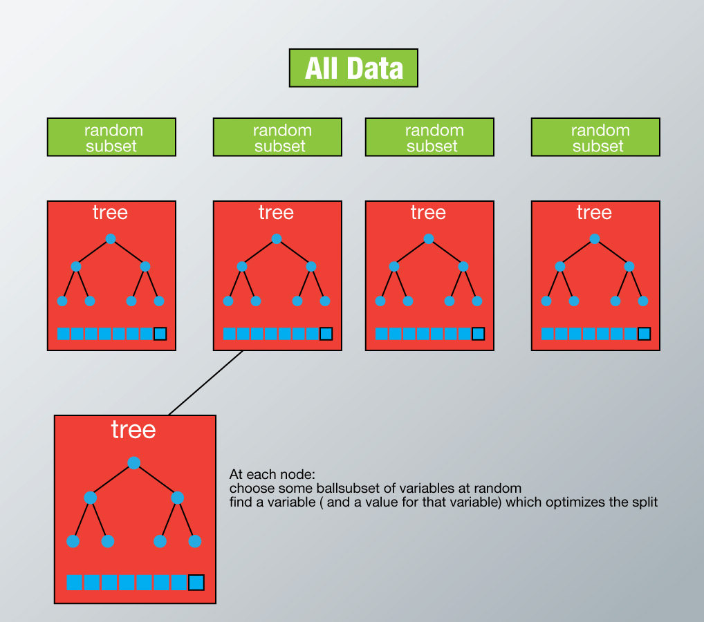
In Random Forest, we grow multiple trees as opposed to a single tree in CART model (see comparison between CART and Random Forest here, part1 and part2). To classify a new object based on attributes, each tree gives a classification and we say the tree “votes” for that class. The forest chooses the classification having the most votes (over all the trees in the forest) and in case of regression, it takes the average of outputs by different trees.

It works in the following manner. Each tree is planted & grown as follows:

1. Assume number of cases in the training set is N. Then, sample of these N cases is taken at random but with replacement. This sample will be the training set for growing the tree.
2. If there are M input variables, a number m
3. Each tree is grown to the largest extent possible and  there is no pruning.
4. Predict new data by aggregating the predictions of the ntree trees (i.e., majority votes for classification, average for regression).

To understand more in detail about this algorithm using a case study, please read this article “Introduction to Random forest – Simplified“.

Advantages of Random Forest

• This algorithm can solve both type of problems i.e. classification and regression and does a decent estimation at both fronts.
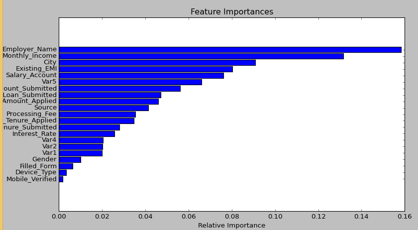
• One of benefits of Random forest which excites me most is, the power of handle large data set with higher dimensionality. It can handle thousands of input variables and identify most significant variables so it is considered as one of the dimensionality reduction methods. Further, the model outputs Importance of variable, which can be a very handy feature (on some random data set).
  
• It has an effective method for estimating missing data and maintains accuracy when a large proportion of the data are missing.
• It has methods for balancing errors in data sets where classes are imbalanced.
• The capabilities of the above can be extended to unlabeled data, leading to unsupervised clustering, data views and outlier detection.
• Random Forest involves sampling of the input data with replacement called as bootstrap sampling. Here one third of the data is not used for training and can be used to testing. These are called the out of bag samples. Error estimated on these out of bag samples is known as out of bag error. Study of error estimates by Out of bag, gives evidence to show that the out-of-bag estimate is as accurate as using a test set of the same size as the training set. Therefore, using the out-of-bag error estimate removes the need for a set aside test set.

Disadvantages of Random Forest

• It surely does a good job at classification but not as good as for regression problem as it does not give precise continuous nature predictions. In case of regression, it doesn’t predict beyond the range in the training data, and that they may over-fit data sets that are particularly noisy.
• Random Forest can feel like a black box approach for statistical modelers – you have very little control on what the model does. You can at best – try different parameters and random seeds!

Python & R implementation

Random forests have commonly known implementations in R packages and Python scikit-learn. Let’s look at the code of loading random forest model in R and Python below:

Python

#Import Library
from sklearn.ensemble import RandomForestClassifier #use RandomForestRegressor for regression problem
#Assumed you have, X (predictor) and Y (target) for training data set and x_test(predictor) of test_dataset
# Create Random Forest object
model= RandomForestClassifier(n_estimators=1000)
# Train the model using the training sets and check score
model.fit(X, y)
#Predict Output
predicted= model.predict(x_test)

R Code

> library(randomForest)
> x <- cbind="" class="c" span="" style="box-sizing: border-box;" x_train="" y_train=""># Fitting model

> fit <- .="" class="c" ntree="500)" pecies="" randomforest="" span="" style="box-sizing: border-box;" x="">> summary(fit) #Predict Output > predicted= predict(fit,x_test)

10. What is Boosting ? How does it work?

Definition: The term ‘Boosting’ refers to a family of algorithms which converts weak learner to strong learners.

Let’s understand this definition in detail by solving a problem of spam email identification:

How would you classify an email as SPAM or not? Like everyone else, our initial approach would be to identify ‘spam’ and ‘not spam’ emails using following criteria. If:

1. Email has only one image file (promotional image), It’s a SPAM
2. Email has only link(s), It’s a SPAM
3. Email body consist of sentence like “You won a prize money of $ xxxxxx”, It’s a SPAM
4. Email from our official domain “Analyticsvidhya.com” , Not a SPAM
5. Email from known source, Not a SPAM

Above, we’ve defined multiple rules to classify an email into ‘spam’ or ‘not spam’. But, do you think these rules individually are strong enough to successfully classify an email? No.

Individually, these rules are not powerful enough to classify an email into ‘spam’ or ‘not spam’. Therefore, these rules are called as weak learner.

To convert weak learner to strong learner, we’ll combine the prediction of each weak learner using methods like:

• Using average/ weighted average
• Considering prediction has higher vote

For example:  Above, we have defined 5 weak learners. Out of these 5, 3 are voted as ‘SPAM’ and 2 are voted as ‘Not a SPAM’. In this case, by default, we’ll consider an email as SPAM because we have higher(3) vote for ‘SPAM’.

How does it work?

Now we know that, boosting combines weak learner a.k.a. base learner to form a strong rule. An immediate question which should pop in your mind is, ‘How boosting identify weak rules?‘

To find weak rule, we apply base learning (ML) algorithms with a different distribution. Each time base learning algorithm is applied, it generates a new weak prediction rule. This is an iterative process. After many iterations, the boosting algorithm combines these weak rules into a single strong prediction rule.

Here’s another question which might haunt you, ‘How do we choose different distribution for each round?’

For choosing the right distribution, here are the following steps:

Step 1:  The base learner takes all the distributions and assign equal weight or attention to each observation.

Step 2: If there is any prediction error caused by first base learning algorithm, then we pay higher attention to observations having prediction error. Then, we apply the next base learning algorithm.

Step 3: Iterate Step 2 till the limit of base learning algorithm is reached or higher accuracy is achieved.

Finally, it combines the outputs from weak learner and creates  a strong learner which eventually improves the prediction power of the model. Boosting pays higher focus on examples which are mis-classified or have higher errors by preceding weak rules.
There are many boosting algorithms which impart additional boost to model’s accuracy. In this tutorial, we’ll learn about the two most commonly used algorithms i.e. Gradient Boosting (GBM) and XGboost.

11. Which is more powerful: GBM or Xgboost?

I’ve always admired the boosting capabilities that xgboost algorithm. At times, I’ve found that it provides better result compared to GBM implementation, but at times you might find that the gains are just marginal. When I explored more about its performance and science behind its high accuracy, I discovered many advantages of Xgboost over GBM:

1. Regularization:
   • Standard GBM implementation has no regularization like XGBoost, therefore it also helps to reduce overfitting.
   • In fact, XGBoost is also known as ‘regularized boosting‘ technique.
2. Parallel Processing:
   • XGBoost implements parallel processing and is blazingly faster as compared to GBM.
   • But hang on, we know that boosting is sequential process so how can it be parallelized? We know that each tree can be built only after the previous one, so what stops us from making a tree using all cores? I hope you get where I’m coming from. Check this link out to explore further.
   • XGBoost also supports implementation on Hadoop.
3. High Flexibility
   • XGBoost allow users to define custom optimization objectives and evaluation criteria.
   • This adds a whole new dimension to the model and there is no limit to what we can do.
4. Handling Missing Values
   • XGBoost has an in-built routine to handle missing values.
   • User is required to supply a different value than other observations and pass that as a parameter. XGBoost tries different things as it encounters a missing value on each node and learns which path to take for missing values in future.
5. Tree Pruning:
   • A GBM would stop splitting a node when it encounters a negative loss in the split. Thus it is more of a greedy algorithm.
   • XGBoost on the other hand make splits upto the max_depth specified and then start pruning the tree backwards and remove splits beyond which there is no positive gain.
   • Another advantage is that sometimes a split of negative loss say -2 may be followed by a split of positive loss +10. GBM would stop as it encounters -2. But XGBoost will go deeper and it will see a combined effect of +8 of the split and keep both.
6. Built-in Cross-Validation
   • XGBoost allows user to run a cross-validation at each iteration of the boosting process and thus it is easy to get the exact optimum number of boosting iterations in a single run.
   • This is unlike GBM where we have to run a grid-search and only a limited values can be tested.
7. Continue on Existing Model
   • User can start training an XGBoost model from its last iteration of previous run. This can be of significant advantage in certain specific applications.
   • GBM implementation of sklearn also has this feature so they are even on this point.

12. Working with GBM in R and Python

Before we start working, let’s quickly understand the important parameters and the working of this algorithm. This will be helpful for both R and Python users. Below is the overall pseudo-code of GBM algorithm for 2 classes:

1. Initialize the outcome
2. Iterate from 1 to total number of trees
  2.1 Update the weights for targets based on previous run (higher for the ones mis-classified)
  2.2 Fit the model on selected subsample of data
  2.3 Make predictions on the full set of observations
  2.4 Update the output with current results taking into account the learning rate
3. Return the final output.

This is an extremely simplified (probably naive) explanation of GBM’s working. But, it will help every beginners to understand this algorithm.

Lets consider the important GBM parameters used to improve model performance in Python:

1. learning_rate
   • This determines the impact of each tree on the final outcome (step 2.4). GBM works by starting with an initial estimate which is updated using the output of each tree. The learning parameter controls the magnitude of this change in the estimates.
   • Lower values are generally preferred as they make the model robust to the specific characteristics of tree and thus allowing it to generalize well.
   • Lower values would require higher number of trees to model all the relations and will be computationally expensive.
2. n_estimators
   • The number of sequential trees to be modeled (step 2)
   • Though GBM is fairly robust at higher number of trees but it can still overfit at a point. Hence, this should be tuned using CV for a particular learning rate.
3. subsample
   • The fraction of observations to be selected for each tree. Selection is done by random sampling.
   • Values slightly less than 1 make the model robust by reducing the variance.
   • Typical values ~0.8 generally work fine but can be fine-tuned further.

Apart from these, there are certain miscellaneous parameters which affect overall functionality:

1. loss
   • It refers to the loss function to be minimized in each split.
   • It can have various values for classification and regression case. Generally the default values work fine. Other values should be chosen only if you understand their impact on the model.
2. init
   • This affects initialization of the output.
   • This can be used if we have made another model whose outcome is to be used as the initial estimates for GBM.
3. random_state
   • The random number seed so that same random numbers are generated every time.
   • This is important for parameter tuning. If we don’t fix the random number, then we’ll have different outcomes for subsequent runs on the same parameters and it becomes difficult to compare models.
   • It can potentially result in overfitting to a particular random sample selected. We can try running models for different random samples, which is computationally expensive and generally not used.
4. verbose
   • The type of output to be printed when the model fits. The different values can be:
     • 0: no output generated (default)
     • 1: output generated for trees in certain intervals
     • >1: output generated for all trees
5. warm_start
   • This parameter has an interesting application and can help a lot if used judicially.
   • Using this, we can fit additional trees on previous fits of a model. It can save a lot of time and you should explore this option for advanced applications
6. presort 
   •  Select whether to presort data for faster splits.
   • It makes the selection automatically by default but it can be changed if needed.

I know its a long list of parameters but I have simplified it for you in an excel file which you can download from this GitHub repository.

For R users, using caret package, there are 3 main tuning parameters:

1. n.trees – It refers to number of iterations i.e. tree which will be taken to grow the trees
2. interaction.depth – It determines the complexity of the tree i.e. total number of splits it has to perform on a tree (starting from a single node)
3.  shrinkage – It refers to the learning rate. This is similar to learning_rate in python (shown above).
4. n.minobsinnode – It refers to minimum number of training samples required in a node to perform splitting

GBM in R (with cross validation)

I’ve shared the standard codes in R and Python. At your end, you’ll be required to change the value of dependent variable and data set name used in the codes below. Considering the ease of implementing GBM in R, one can easily perform tasks like cross validation and grid search with this package.

> library(caret)

> fitControl <- span=""> trainControl(method = "cv",
                           number = 10, #5folds)

> tune_Grid <- span="">  expand.grid(interaction.depth = 2,
                            n.trees = 500,
                            shrinkage = 0.1,
                            n.minobsinnode = 10)

> set.seed(825)
> fit <- span=""> train(y_train ~ ., data = train,
                 method = "gbm",
                 trControl = fitControl,
                 verbose = FALSE,
                 tuneGrid = gbmGrid)

> predicted= predict(fit,test,type= "prob")[,2] 

GBM in Python

#import libraries

from sklearn.ensemble import GradientBoostingClassifier #For Classification
from sklearn.ensemble import GradientBoostingRegressor #For Regression

#use GBM function

clf = GradientBoostingClassifier(n_estimators=100, learning_rate=1.0, max_depth=1)
clf.fit(X_train, y_train)

13. Working with XGBoost in R and Python

XGBoost (eXtreme Gradient Boosting) is an advanced implementation of gradient boosting algorithm. It’s feature to implement parallel computing makes it at least 10 times faster than existing gradient boosting implementations. It supports various objective functions, including regression, classification and ranking.

R Tutorial: For R users, this is a complete tutorial on XGboost which explains the parameters along with codes in R. Check Tutorial.

Python Tutorial: For Python users, this is a comprehensive tutorial on XGBoost, good to get you started. Check Tutorial.

14. Where to practice ?

Practice is the one and true method of mastering any concept. Hence, you need to start practicing if you wish to master these algorithms.

Till here, you’ve got gained significant knowledge on tree based models along with these practical implementation. It’s time that you start working on them. Here are open practice problems where you can participate and check your live rankings on leaderboard:

For Regression: Big Mart Sales Prediction

For Classification: Loan Prediction

End Notes

Tree based algorithm are important for every data scientist to learn. In fact, tree models are known to provide the best model performance in the family of whole machine learning algorithms. In this tutorial, we learnt until GBM and XGBoost. And with this, we come to the end of this tutorial.

We discussed about tree based modeling from scratch. We learnt the important of decision tree and how that simplistic concept is being used in boosting algorithms. For better understanding, I would suggest you to continue practicing these algorithms practically. Also, do keep note of the parameters associated with boosting algorithms. I’m hoping that this tutorial would enrich you with complete knowledge on tree based modeling.

Did you find this tutorial useful ? If you have experienced, what’s the best trick you’ve used while using tree based models ? Feel free to share your tricks, suggestions and opinions in the comments section below.

You can test your skills and knowledge. Check out Live Competitions and compete with best Data Scientists from all over the world.